When we want to see the text of a specific content in Excel and display it, we need to color the cells that contain the specified content.
Step:
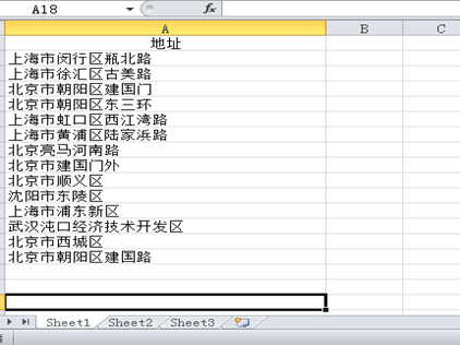
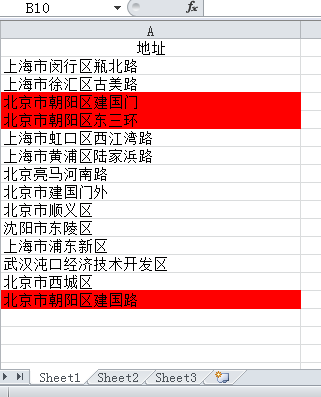
For example: The information displayed in Excel in the figure, we need to find all the information of “北京市朝阳区” and fill in the red.
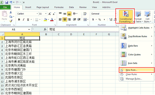
- Choose the Conditional Formatting tool: Select this column of information and select conditional formatting-new rule in the toolbar.
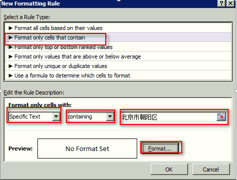
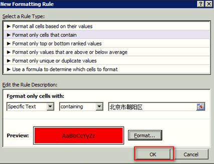
- New formatting rule: In the dialog box for new formatting rules, select format only cells, edit the format under Edit Rule description, select specific text in the selection box,containing, in the Description box, enter “北京市朝阳区” and click “format”;
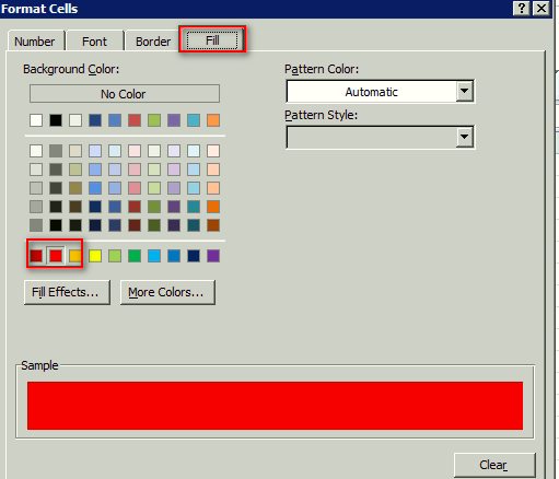
- Format Cells: After the previous Steps, a pop-up box with format cells appears. Select Fill, click on the color red that we want to fill in the background color display below the fill, the example will appear red color bar, then click “OK”, the page returns to “new format rule” The Bullet box, click “OK”;
- After the completion of the above Steps, contains the contents of 北京市朝阳区 are filled with red
See you next week.
