Icon Set is a very useful tool in conditional formatting. With it, you can easily add small icons in cells to highlight data characteristics and make the report more intuitive to the reader.

Example
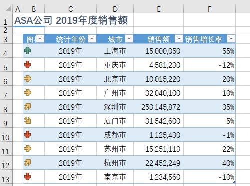
Let us use a common sales data report as an example. Highlight sales growth with colored arrow icons, so reader can immediately find the row of data they care about:
The green arrows represent good sales growth.
The yellow arrows represent medium sales growth.
The red arrows represent bad sales growth.
Steps
We don’t need to manually calculate sale growth and add the arrow icons, we just need to setup Icon Set, and Excel will take care of the rest for us.
1、Create the first column
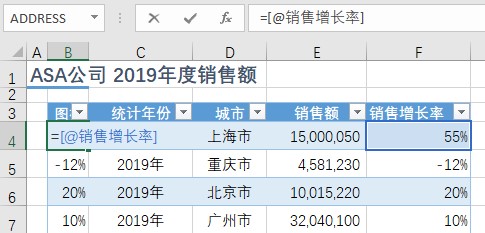
Let us insert a new column named Legend before the “statistics year” column. Then quote the “Sales Growth Rate” column.
2、Setup in Conditional formatting
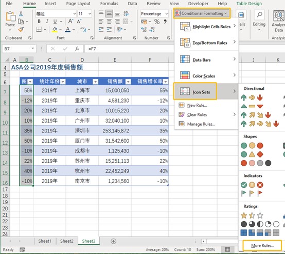
First, in Excel sheet, select all the cells that determine the growth. Click “Conditional Formatting” and select “Icon Sets” then click “More Rules”.
3、Setup Rules
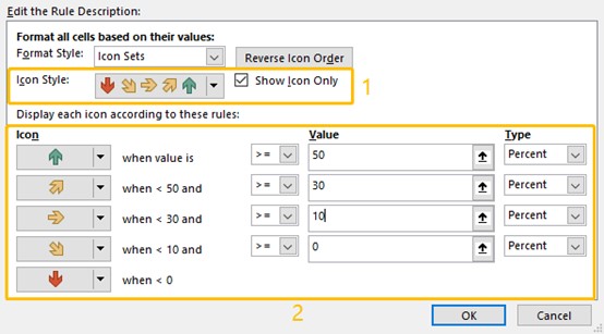
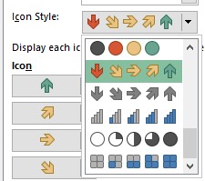
Select the icon style, then setup the rules. In which range which icon should be displayed.
As we just display icon in first column, so check the“Show Icon Only”.
After finish setup rules, click “OK”to see the effect.
At the Last
Please note that, the Icon Sets only can setup 5 icons, but it is generally enough.
If you’re interested in making your report stand out from the crowd, just try it!
