Hello everyone, today We continue to share some simple and practical uses of function formulas.
Sum in merged cells
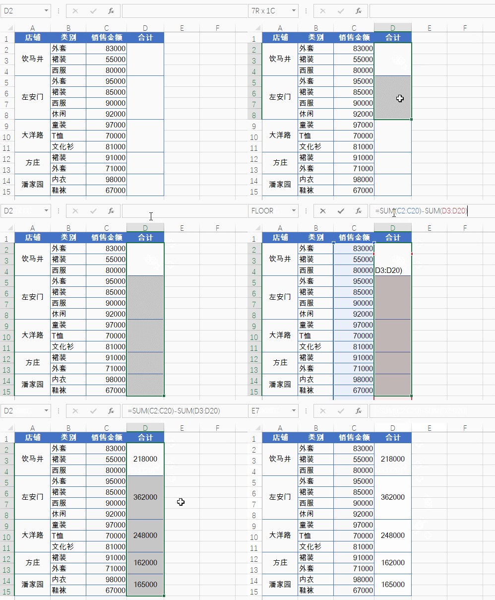
As shown in the picture below, it needs to count the sales amount for each store.
At the same time, select the D2:D10 , enter the formula and press Ctrl+ Enter
=SUM(C2:C20)-SUM(D3:D20)

SUM(C2:C20) is the SUM of the current row and the following C column. SUM(D3:D20) is the SUM of all the categories other than this category.
Subtract these two totals and you get the sum of this category.
Limit input duplicate data
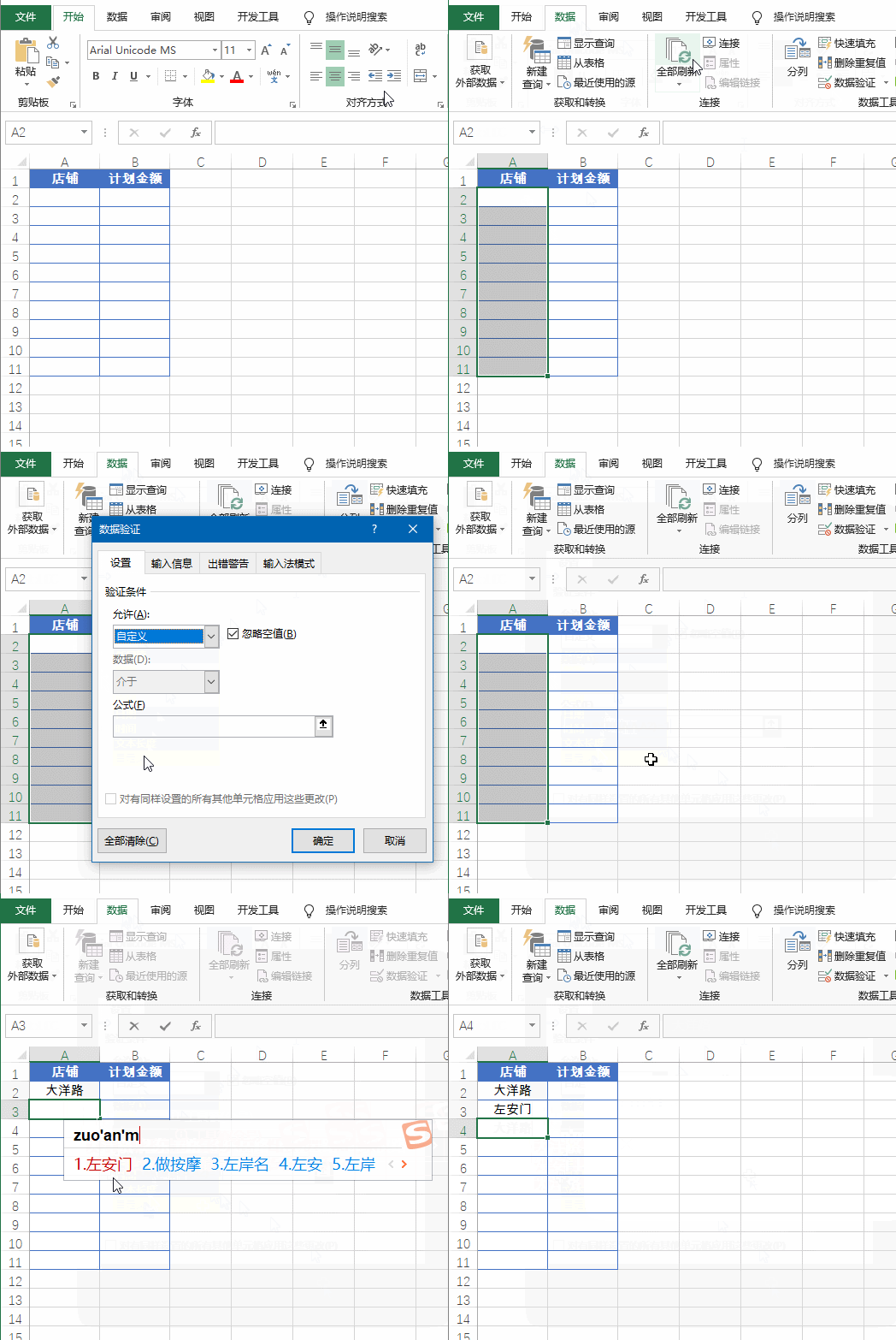
Select the A2:A10 cell area for which you want to enter data. Click “Data”->”Data Validation”
Select “Custom” in Allow, then input the formula:
=COUNTIF(A:A,A2)=1

Highlight duplicate data
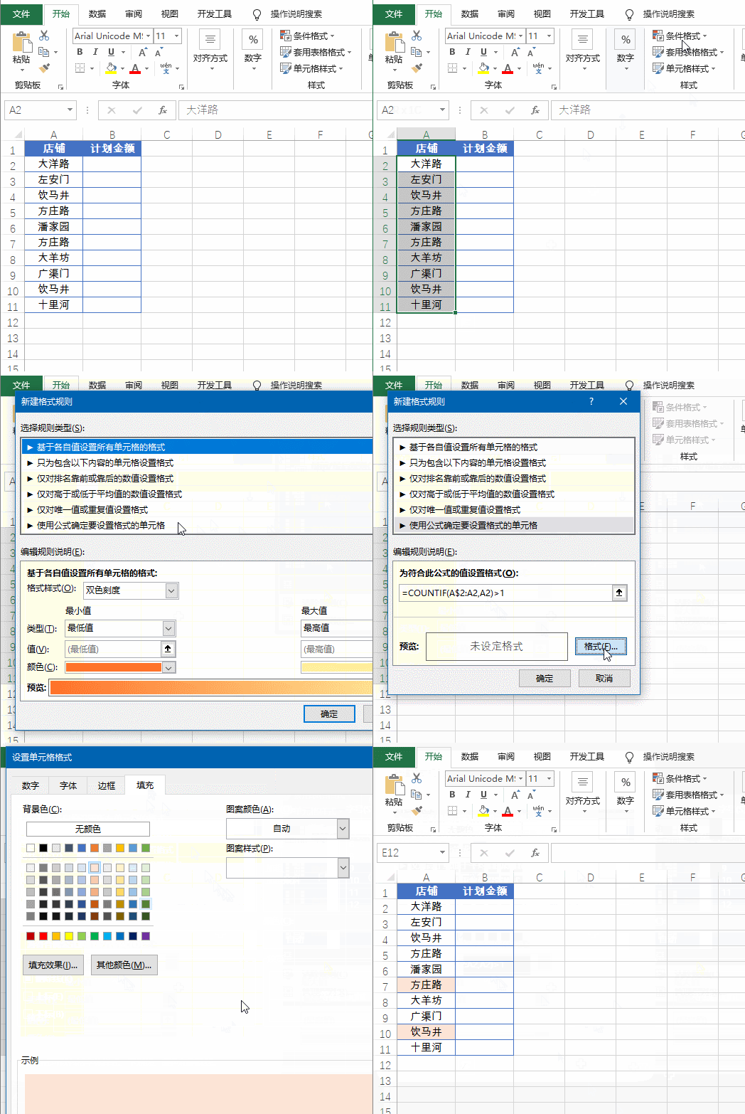
Select the area of A2:A10 cells for which you have entered data and create a new format rule.
The formula is
=COUNTIF(A$2:A2,A2)>1
Set the format of the highlight

Use XLOOKUP to look up data
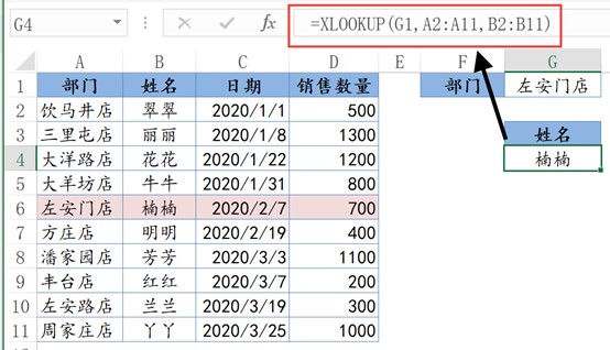
As shown in the picture below, query the department in column A based on G1 and return the name of the person in charge corresponding in column B.
If you’re using Excel 2021 or Office 365, you can use this formula:
=XLOOKUP(G1,A2:A11,B2:B11)

The first parameter is the content of the query, and the second parameter is the query area. You only need to select a column for the query area. The third argument is to return the contents of the column, again just by selecting a column.
The formula looks for the department specified in cell G1 in cell A2:A11 and returns the corresponding name in cell B2:B11.
That’s all for today, Have a great weekend!
